Rows, Columns, and What They Cost

The first piece followed George Stigler's diet problem from a hand-built answer to a proof. In 1945 Stigler asked for the cheapest combination of foods that would meet nine minimum nutritional requirements. He had 77 foods to choose from, no general method for finding the minimum, and enough economic instinct to get remarkably close by inspection.

His basket cost $39.93 a year. Two years later, by George Dantzig's later account, nine clerks at the National Bureau of Standards spent about 120 man-days putting the full problem through the new simplex method. They found a diet costing $39.69. The twenty-four cents was not what justified the labour. The calculation also produced nine shadow prices which, multiplied by the nutrient requirements and added, matched the cost of the diet. The basket and the prices certified one another: no cheaper diet satisfying all nine requirements existed.

That established what optimal meant, but it left the machine closed. What did the simplex method actually receive, and what did the size of that input say about the work ahead? Start with Stigler's table of 77 foods and nine nutrients. To turn it into the matrix an optimiser uses, put one nutrient requirement in each row and one food choice in each column. The result has nine rows, 77 columns and 693 cells.

Each cell is a coefficient: how much of that row's nutrient one dollar spent on that column's food supplies. A non-zero means the choice affects the requirement; a zero means Stigler's table records no contribution. There are 570 non-zero cells. Density is simply the share of all cells that are non-zero: 570 divided by 693, or 82.3 per cent.

That gives us four different descriptions before an algorithm has done anything. Rows are promises to keep. Columns are choices available. The rectangle contains 693 possible relationships; 570 are present; 82.3 per cent is the fraction present. None of those numbers is a difficulty score. A model can be enormous and routine, or fit on one page and ruin your week.

Ninety-eight models on the same shelf

To decide whether 82.3 per cent is unusual, we need something to compare it with. Netlib is a public archive of numerical software, data and test problems. Its linear-programming directory is a long-standing benchmark collection: a common shelf of models that developers can give to different solver programs and check whether they reach the recorded answers.[1] Benchmark means a repeatable test set, not a representative sample of every model used in industry.

Each problem on that shelf has a short file name. AFIRO is the smallest entry in the summary table, contributed from Stanford's Systems Optimization Laboratory: 28 rows by 32 columns. The archive records its provenance but does not explain what the name expands to or what application, if any, sits behind it. STOCFOR3 is documented more fully. It is the third and largest of a family of seven-period forestry-planning models in which forest fires are random: 16,676 rows by 15,695 columns. AFIRO and STOCFOR3 are not algorithms or technical terms. They are two named test files, one small and one large.

Netlib's summary currently lists 98 such linear programs. Its bookkeeping includes the objective—the row of costs—in the row and non-zero totals, while leaving out auxiliary columns that solvers add when turning inequalities into equations. To compare Stigler on the same terms, add his all-ones cost row to the nine nutrient rows. The matrix then has 647 non-zeros in 770 cells: 84.0 per cent, or 8.4 non-zeros per decision column.

Across the 98 Netlib entries, the median is 4.8 non-zeros per column. The middle half runs from 4.0 to 7.4. Stigler is on the coupled side, but it is not an alien object. Its spectacular density comes mainly from having only ten rows.

The larger Netlib models make the denominator grow while the local coupling barely moves. Among the 27 instances with fewer than 100,000 matrix cells, the median column touches 5.1 rows. Among the ten with more than ten million cells, it touches 5.0. These are measurements of this old benchmark collection, not a law of industrial optimisation, but they make the arithmetic trap visible: if each new decision continues to touch about five constraints, percentage density falls automatically as the number of rows rises.

The zeros are not empty storage waiting to be filled. They say that a decision made over here has no direct effect on a promise made over there. A large network model can be manageable because locality keeps most of those relationships absent. A much smaller matrix can be painful because almost everything talks to everything else.

From the table to a linear program

The same bookkeeping becomes algebra on one line:

Here x has 77 entries, one daily expenditure for each food. The vector c is unusually simple: 77 ones, because the objective is just the sum of those expenditures. The matrix A has nine rows and 77 columns, one nutrient yield for every nutrient-food pair. The vector b holds the nine minimum daily allowances.

The two matrix dimensions do opposite jobs. A column is a choice the optimiser may use. Add a food and the feasible set gains a direction. A row is a promise the answer must keep. Add a nutrient minimum and the feasible set is cut down. Both operations make a file larger. One creates freedom and the other removes it.

To run the simplex method, write the inequalities as equations by subtracting a non-negative surplus vector s:

There are now nine equations and 86 columns: 77 foods plus nine surpluses. A basis selects nine of those 86 columns. The crude combinatorial ceiling on the selections to inspect is therefore

possible column sets. At one microsecond each, checking them all would take 5.3 days. The solve on my laptop takes milliseconds.

Those 459 billion selections are not 459 billion bases or vertices. Many are singular, many produce an infeasible point, and degeneracy lets several genuine bases describe the same vertex. The number is still useful because it says what the algorithm refuses to do. The simplex method moves between adjacent feasible bases and uses reduced costs to choose a direction. It does not scan the catalogue.[2]

This is why “77 variables” is not an account of the computation. The rectangle is 9 by 77, the standard-form matrix is 9 by 86, the nine-column selection count is almost half a trillion, and the path actually visited is tiny. Four true descriptions, four different numbers.

Why the answer contains five foods

The same basis explains the strange economy of the optimal basket.

The fundamental theorem of linear programming is existential: if a standard-form LP has an optimum, at least one optimal solution is basic.[3] A basis here has nine columns, so an optimal basic solution has at most nine positive variables among the 77 foods and nine surpluses together. It may have fewer than nine positive variables because a basic variable is allowed to equal zero. That is degeneracy, and it is common.

Four nutrient constraints are loose at the optimum. The diet supplies more protein, iron, thiamine and niacin than their required floors. Their four surplus variables are therefore positive, and every positive variable must be basic. Four of the nine possible positive positions are already occupied. At most five foods remain.

The computed answer uses exactly five: wheat flour, cabbage, spinach, dried navy beans and beef liver. Offer the model ten thousand more foods while keeping the same nine nutritional floors and there will still exist an optimal basic answer using no more than nine foods, and no more than five if the same four floors remain loose.

The dual makes the other half of the pattern visible:

Complementary slackness pairs the two solutions. If a food appears in the basket, the corresponding dual inequality is tight: the nutrients bought with one dollar of that food are priced at exactly one dollar. If a nutrient floor is exceeded, its shadow price is zero.[4] In this particular solution the five foods are positive, five nutrient prices are positive and four are zero. The matching counts are a feature of this non-degenerate pair, not a general identity between foods and prices.

There is another qualification worth keeping. The theorem says that a sparse optimal vertex exists. It does not say every optimum is sparse. If the objective is flat along a face, a dense mixture of optimal vertices is optimal too. The simplex method normally returns a vertex; an interior-point solver can approach a point in the face and may cross over to a basis afterward. If a buyer wants a balanced allocation across suppliers, that preference belongs in the model. The unadorned LP has no reason to invent it.

The pattern behind the count

Non-zeros are a better first question than rows times columns, but they are still only a first question.

Both major LP algorithm families repeatedly solve linear systems. A simplex implementation factorises a basis matrix and updates that factorisation as columns enter and leave. A primal-dual interior-point implementation solves a Newton system at every iteration. The starting matrices are sparse. Their factors need not be.

Elimination creates new non-zeros where the original matrix had zeros. Sparse linear algebra calls this fill-in. The amount depends on the pattern, the order in which rows and columns are eliminated and, for unsymmetric systems, numerical pivoting—which is why solvers spend real effort choosing permutations.[5] Two matrices can have the same dimensions and exactly the same number of non-zeros, yet produce factors with very different sizes.

A small graph gives the intuition. Eliminating a node forces its surviving neighbours to become connected to one another. Remove the hub of a star first and the leaves become a clique. Remove the leaves first and almost nothing happens. The node and edge counts did not change before elimination; the order changed what had to be created during it.

So the first useful inspection of a slow model is not “how many variables?” It is the distribution of non-zeros by row and column, the block or network structure, the numerical scaling, and what presolve removes. None of these alone predicts runtime. Together they are closer to the object the solver actually sees than m × n.

Polynomial and fast are different claims

Linear programming owns one of the better misunderstandings in applied mathematics. The simplex method is famously fast. Linear programming is polynomial-time. The two sentences refer to different algorithms.

Klee and Minty constructed a distorted cube in 1972 on which Dantzig's original pivot rule visits every one of its 2ⁿ vertices.[6] Related lower bounds exist for several other pivot rules. This is a worst-case statement about those paths through the polytope, not a prediction for Stigler's diet or a modern solver.

Khachiyan supplied the first polynomial-time algorithm for LP in 1979 using the ellipsoid method.[7] Its running time is polynomial in the binary input length, so the sizes of the coefficients matter. That is usually called weakly polynomial. Karmarkar's 1984 projective method then opened the modern interior-point route while retaining a polynomial bound.[8] Whether general LP has a strongly polynomial algorithm, with a number of arithmetic operations independent of coefficient bit-length, remains open. Smale put it ninth on his list of problems for this century.[9]

Worst-case theory and measured solver progress can both be true. Koch and co-authors compared LP and MILP software from 2001 with 2020-era codes. On the instances both generations could solve, they estimate a factor of about 20 from hardware and nine from LP algorithms, roughly 180 in combination. They also warn that the averages have high variance and omit much of the progress, because many instances the old codes cannot finish at all are now solved in seconds.[10]

No single line in that history says which algorithm will win on the next model. Modern solvers keep simplex and barrier methods because structure decides. “Polynomial” is a guarantee about how a bound scales. “Fast” is an observation made on a machine, a model family and a tolerance.

Four convex dialects, one kind of proof

Linear objectives and constraints are only the first rung. The other common convex forms buy more expressive syntax while keeping a route to a primal-dual certificate.

The table mixes one problem form, QP, with cone-defined classes on purpose. A convex quadratic can be rewritten with a rotated second-order cone; an SOCP can be written as an SDP. This gives a representational ladder, not an instruction to send every LP to an SDP solver. A specialised algorithm lower down will usually exploit structure the general reformulation hides.

Interior-point theory makes part of the price precise. The standard barrier for one non-negative orthant in n dimensions has parameter n. A single second-order-cone block has parameter 2, independent of that block's dimension. A positive-semidefinite cone of k by k matrices has parameter k.[11] Parameters add across cone blocks and help bound the number of Newton steps. They do not measure runtime. Forming and factorising one SDP Newton system can cost far more than taking one LP step.

Markowitz sits on the second rung when Σ is positive semidefinite: minimise w^TΣ w under a return target and a budget. Under the factor model and uncertainty sets specified by Goldfarb and Iyengar, robust versions of that portfolio problem become SOCPs.[12] Change the uncertainty set, especially by putting a general semidefinite condition directly on the covariance, and the reformulation changes with it. The geometry chosen for what you do not know becomes part of the computational model.

The certificate also needs a qualification. LP strong duality is unusually well behaved. In general conic problems, a condition such as strict feasibility is what makes the primal and dual optima meet; semidefinite programs can exhibit a positive gap or fail to attain an optimum when regularity fails.[4] Convexity keeps the local-versus-global promise. It does not waive the hypotheses of duality.

Everything so far still lives on Rockafellar's cooperative side of the watershed. The matrix may be large, sparse, badly ordered or expressed through a more expensive cone, but the feasible set has no holes. The next piece adds one innocent-looking instruction: this warehouse is open or closed; this gene is deleted or it is not. Half a warehouse is no longer a point you can visit. The rows and columns remain, and the proof becomes a gap.

Data and code

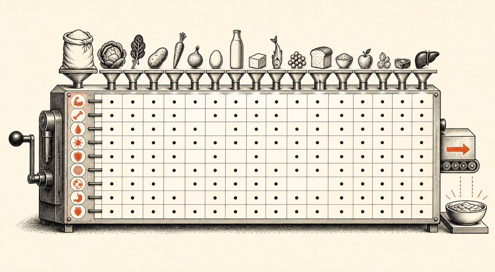
The matrix calculations and both figures are reproducible in the Post 2 folder of github.com/Denis-Joly/what-optimal-means. The optimal diet itself is solved in the Post 1 folder; Figure 2 uses its four-surplus, five-food result to explain the basis structure.

analyze_structure.py reads the Stigler table used in the first piece and a dated copy of Netlib's official summary. It prints the standard-form basis count, the matrix statistics and every threshold used above. make_figures.py turns those statistics and the documented Post 1 solution into standalone SVGs, responsive article fragments and a local interactive demo; article-viz.js adds the metric switch and exact-value explorer without a charting library. Netlib's convention of including the objective row is kept in the code rather than corrected silently.

The comparison has limits. Netlib is a classic benchmark set assembled from older academic and operational models, not a random sample of today's supply chains. The split at 100,000 and ten million cells is descriptive. It shows that non-zeros per column stay almost unchanged within this collection; it does not claim a universal constant.

References

1. Netlib, linear-programming directory and LP/DATA problem summary table. The directory describes the collection as test problems in MPS, the old machine-readable interchange format for linear programs. The table currently lists 98 problems, names AFIRO's Stanford source, and describes STOCFOR1–3 as Gus Gassmann's seven-period forestry models with random forest fires. Its notes state that row and non-zero counts include the cost row, while column and non-zero counts exclude slack and surplus columns. The statistics here are my calculations from that table, downloaded 11 August 2026.
2. George B. Dantzig, Linear Programming and Extensions (Princeton University Press, 1963), especially the geometric and revised-simplex treatments.
3. David G. Luenberger and Yinyu Ye, Linear and Nonlinear Programming, 3rd ed. (Springer, 2008), §2.3–2.4, pp. 19–21. The theorem guarantees an optimal basic feasible solution when an optimum exists.
4. Stephen Boyd and Lieven Vandenberghe, Convex Optimization, 2004. Complementary slackness is §5.5.2; certificates and strong duality are treated in chapter 5.
5. Timothy A. Davis, Sivasankaran Rajamanickam and Wissam M. Sid-Lakhdar, “A survey of direct methods for sparse linear systems”, Acta Numerica 25 (2016): 383–566. Fill-in and permutations are introduced at pp. 8–9.
6. Victor Klee and George J. Minty, “How Good Is the Simplex Algorithm?”, in Inequalities III (Academic Press, 1972), 159–175.
7. Leonid G. Khachiyan, “A Polynomial Algorithm in Linear Programming,” Soviet Mathematics Doklady 20 (1979): 191–194.
8. Narendra Karmarkar, “A New Polynomial-Time Algorithm for Linear Programming”, Combinatorica 4 (1984): 373–395.
9. Stephen Smale, “Mathematical Problems for the Next Century,” The Mathematical Intelligencer 20 (1998): 7–15.
10. Thorsten Koch, Timo Berthold, Jaap Pedersen and Charlie Vanaret, “Progress in Mathematical Programming Solvers from 2001 to 2020”, EURO Journal on Computational Optimization 10 (2022): 100031.
11. Boyd and Vandenberghe, Convex Optimization, examples 11.5–11.7, pp. 597–598; Aharon Ben-Tal and Arkadi Nemirovski, Lectures on Modern Convex Optimization (SIAM, 2001), lecture 4.
12. Donald Goldfarb and Garud Iyengar, “Robust Portfolio Selection Problems”, Mathematics of Operations Research 28, no. 1 (2003): 1–38.